RAG - Retrieval Augmented Generation
A Guide to understand and build RAG application, with Embedding, Sentence BERT, Vector Database, and LLMs
Introduction
AI: I am sorry, i can not provide you the answer without context or I was trained on before date.
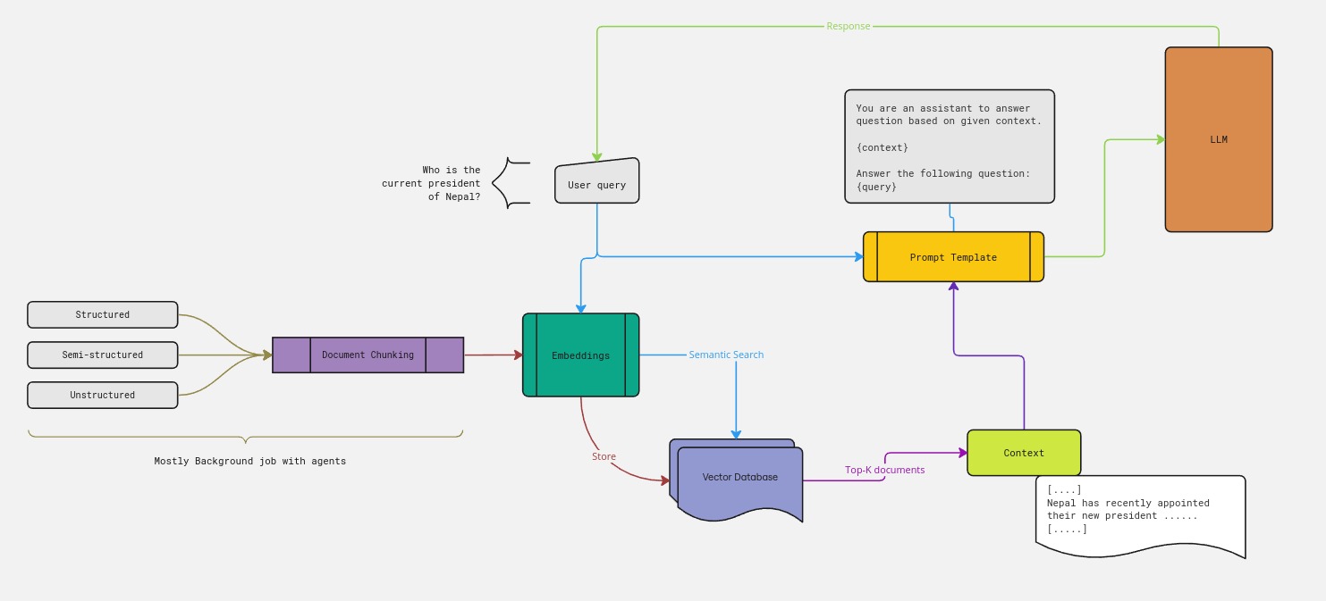
Retrieval Augmented Generation (RAG) combines retrieval-based and generative models in natural language processing to produce contextually relevant and coherent responses by first retrieving relevant passages or documents and then using them to guide the generative model.
At its core, Retrieval Augmented Generation is a fusion of two fundamental approaches in NLP:
-
Retrieval-Based Models: These models excel at retrieving relevant information from large corpora of text based on a given query or context. They leverage techniques like similarity search, or advanced methods such as dense retrieval with neural networks to efficiently fetch passages that are most likely to contain the desired information. In another words, finding most relevant documents for a input query based on specified algorithm (cosine similarity, or any distnace metrics).
-
Generative Models: On the other hand, generative models, particularly those based on transformers like GPT (Generative Pre-trained Transformer), have demonstrated remarkable proficiency in generating human-like text. They operate by predicting the next word or token in a sequence based on the preceding context, often trained on vast amounts of text data.
Retrieval Augmented Generation seeks to harness the strengths of both these approaches by integrating retrieval-based systems into the generative pipeline. The basic idea is to first retrieve a set of relevant passages or documents from a knowledge source (such as a large text corpus or a knowledge graph) and then use these retrieved contexts to guide the generative model in producing a more informed and contextually appropriate response.
Here’s how the process typically unfolds:
-
Retrieval: Given an input query or context, a retrieval-based model is employed to fetch a set of relevant documents or passages from a knowledge base. This retrieval step is crucial for providing the generative model with a rich source of contextual information.
-
Generation: The retrieved passages serve as the context for the generative model, which then generates a response based not only on the original input but also on the retrieved knowledge. By incorporating this additional context, the generative model can produce responses that are more coherent, informative, and contextually relevant.
-
Ranking: In some implementations, a ranking mechanism may be employed to select the most suitable response among multiple candidates generated by the generative model. This step ensures that the final output is of the highest quality and relevance.
The beauty of Retrieval Augmented Generation lies in its ability to combine the depth of knowledge retrieval with the creativity of generative models, resulting in responses that are not only fluent and coherent but also grounded in factual accuracy and contextual understanding. This approach has numerous applications across various domains, including question answering, conversational agents, content generation, and more.
Large Language Models
Large Language Models (LLMs) stand as marvels of mathematical ingenuity intertwined with cutting-edge technology. At their core, LLMs rely on intricate neural network designs, often built upon the transformative Transformer architecture. These models boast layers of attention mechanisms, allowing them to adeptly capture intricate linguistic nuances and dependencies within text. One key mathematical concept underpinning LLMs is the notion of attention mechanisms, particularly prevalent in architectures like the Transformer model. Attention mechanisms enable the model to weigh the importance of different words or tokens in a sequence, allowing it to focus on relevant information while filtering out noise. This process involves matrix operations and vector manipulations, where attention scores are computed through dot products and softmax functions, creating a weighted representation of the input.
Additionally, LLMs leverage sophisticated optimization algorithms, such as stochastic gradient descent and its variants, to iteratively adjust model parameters during training, minimizing a loss function that quantifies the disparity between predicted and actual text. Through these mathematical intricacies, LLMs harness the power of data and computation to transcend the boundaries of language understanding and generation.
For instance, P ["Nepal" | "Kathmandu is a city in ____"]. In this example, pormpt : "Kathmandu is a city in" and prediction of LLM model token: "Nepal". The LLM model simply spits out the probability of each word in predefined vocabulary. It accquires the knowledge such as context, relationship via training.
List of some LLMs:
- GPT-3.5 and GPT-4 by OpenAI: These models power applications like ChatGPT and Microsoft Copilot².
- PaLM by Google: A commercial LLM.
- Gemini by Google: Currently used in the chatbot of the same name.
- Grok by xAI: An intriguing LLM.
- LLaMA family of open-source models by Meta.
- Claude models by Anthropic.
- Mistral AI’s open-source models.
- DBRX by Databricks: An open-source LLM².
Fine Tuning
Fine-tuning is the process of taking a pre-trained model and further training it on a specific task or dataset to enhance its performance for that particular objective. Essentially, fine-tuning enables the adjustment of the parameters of the pre-trained model to adapt it to the intricacies of the target task or domain.
Fine-tuning techniques:
-
LoRA (Low Rank Adaption of LLM): LoRA is a fine-tuning technique designed specifically for Large Language Models (LLMs), such as GPT models. It focuses on efficiently adapting pre-trained LLMs to new tasks while mitigating the risk of catastrophic forgetting, which occurs when the model forgets previously learned knowledge while learning new information. LoRA achieves this by introducing low-rank adaptations to the model’s parameters during fine-tuning. By adjusting the rank of parameter matrices in the LLM, LoRA allows for more efficient adaptation to new tasks without significantly increasing computational overhead.
-
QLoRA (Quantized Low Rank Adaption of LLM): QLoRA builds upon the principles of LoRA while introducing quantization to further optimize the fine-tuning process. In QLoRA, the low-rank adaptations of LLM parameters are quantized into a discrete set of values. This quantization serves to stabilize training and reduce memory requirements, making fine-tuning more computationally efficient. By combining low-rank adaptation with quantization, QLoRA enables effective fine-tuning of LLMs on diverse tasks with minimal computational overhead.
These techniques represent innovative approaches to fine-tuning LLMs for specific tasks, offering efficient solutions to adapt pre-trained models to new domains while preserving previously learned knowledge.Techniques like LoRA and QLoRA can unlock the full potential of LLMs across a wide range of natural language processing tasks and applications.
Fine-tuning and Pretraining a LLM is prohbitively expensive.
Prompt Engineering
Prompt engineering involves crafting tailored instructions or queries to guide AI models towards accurate and contextually relevant outputs. For instance, in a conversational AI system designed to provide movie recommendations based on user preferences, a good prompt might include specific criteria such as genre, release year, and preferred actors, such as “Recommend a Nepali movie released in the past five years starring either Bipin Karki or Dayahang Rai.” This nuanced instruction provides the AI model with clear guidance on the user’s preferences, enabling it to generate highly relevant and personalized recommendations, showcasing the intricate nature of prompt engineering in AI applications.
The general format:
-
Instructions:You are an assistant ................. -
Context:This is context ...... -
Question/Query:Your question ..... -
Answer:LLM generated response
RAG Pipeline
RAG Pipeline consists of many components.

Embedding Vectors
In natural language processing (NLP), embedding refers to the process of representing words or tokens as numerical vectors in a continuous vector space. These vectors capture semantic relationships between words, enabling NLP models to understand and process textual data more effectively. BERT (Bidirectional Encoder Representations from Transformers) is a powerful model that generates word embeddings with rich contextual information.
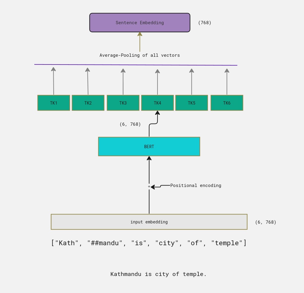
Let’s illustrate embedding with the example text "Kathmandu is city of temple" using BERT:
In BERT, each word in the sentence is tokenized and represented as a vector. For instance, the word "Kathmandu" is tokenized into individual subwords or tokens, such as ["Kath", "##man", "##du"]. Each token is embedded into a high-dimensional vector space.
In the case of “Kathmandu is city of temple,” BERT captures the contextual information of each token by considering its surrounding tokens. So, the embedding for "Kath" might be influenced by the tokens "is" and "city," indicating its context within the sentence.
Similarly, the embedding for "city" would capture its relationship with "Kathmandu" and "temple" in the sentence, enabling BERT to understand that "city" is associated with both "Kathmandu" and "temple" in this particular context.
By generating embeddings that encode contextual information, BERT enables NLP models to grasp the nuanced meanings of words in different contexts. These embeddings serve as input to downstream tasks, allowing the model to make accurate predictions or generate relevant outputs based on the semantic information captured in the embeddings.
Sentence Embedding
Sentence embedding refers to the process of representing entire sentences or phrases as numerical vectors in a continuous vector space, capturing their semantic meaning and context. Let’s explore sentence embedding using the example “Kathmandu is city of temple.”
In sentence embedding, the sentence “Kathmandu is city of temple” would be tokenized into individual words or subwords and processed to generate a single vector representation that encapsulates its semantic meaning and context.
Using a pre-trained language model like BERT or Universal Sentence Encoder, each word or subword in the sentence is converted into a vector representation, and these individual embeddings are combined or aggregated to produce a final vector representation for the entire sentence.
For example, the sentence “Kathmandu is city of temple” might be tokenized into the following subwords: ["Kath", "##mandu", "is", "city", "of", "temple"]
Each of these subwords is then embedded into a high-dimensional vector space. The embedding for the entire sentence is computed by aggregating or combining these individual subword embeddings, typically using techniques like averaging or pooling.
The resulting sentence embedding captures the semantic meaning and context of the entire sentence “Kathmandu is city of temple” in a continuous vector representation. This embedding can then be used as input to downstream NLP tasks such as sentiment analysis, text classification, or semantic similarity comparison between sentences, allowing NLP models to make accurate predictions or generate relevant outputs based on the semantic information encoded in the embedding.

How does the model know if two sentence have similar meaning ?
One of the popular method to find relationship between sentences (vectors in nutshell) is cosine similarity score. It measures the the angle between two vectors. A small angle results in high score that is also a highly similar vector.
Given two n-dimensional vectors of attributes, $A$ and $B$, the cosine similarity, $cos(θ)$, is represented using a dot product and magnitude as
\[S_C(A,B)\] \[cos(\theta) = \frac{A \cdot B}{\|A\| \|B\|} = \frac{\sum_{i=1}^n A_i B_i}{\sqrt{\sum_{i=1}^n A^2_n} \cdot \sqrt{\sum_{i=1}^n B^2_n}}\]Yet, how to teach BERT to use desired similarity metrics like cosine and assure two sentences produce the similar result?
Sentence BERT
Sentence BERT (SBERT) is a variant of the BERT (Bidirectional Encoder Representations from Transformers) model specifically designed for generating high-quality sentence embeddings. Unlike traditional BERT, which operates at the word level, SBERT processes entire sentences or phrases to generate embeddings that capture the semantic meaning and context of the input text.
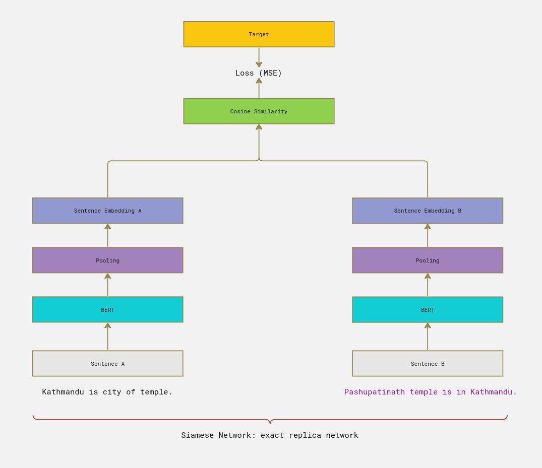
SBERT achieves this by fine-tuning the BERT architecture on a variety of sentence-level tasks, such as sentence similarity, paraphrase identification, and natural language inference. During training, SBERT learns to encode the semantic similarity between pairs of sentences, allowing it to generate embeddings that effectively capture the meaning of entire sentences.
One key innovation of SBERT is the use of siamese or triplet network architectures, where multiple copies of the BERT model share weights and are trained to optimize a similarity metric between sentence pairs. This encourages SBERT to learn representations that are invariant to certain transformations (e.g., word order or paraphrasing) while emphasizing differences between dissimilar sentences.
SBERT embeddings have demonstrated superior performance in various NLP tasks requiring sentence-level understanding, such as semantic textual similarity, text classification, and information retrieval.

Vector Database
A vector database is a type of database that stores data in the form of vectors, typically numerical representations of objects or documents in a high-dimensional (predefined) vector space. These databases are designed to efficiently store and retrieve vector data, enabling various applications such as similarity search, recommendation systems, and information retrieval.
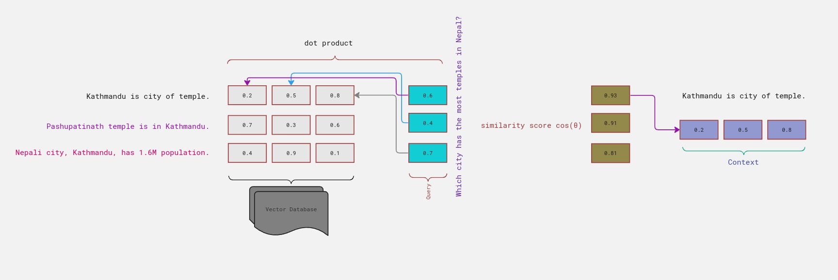
Suppose we have a collection of documents, each represented as a numerical vector in a high-dimensional space. These vectors capture the semantic meaning and features of the documents.
For simplicity, let’s consider a small collection of three documents represented by their vectors:
Documents: $A, B, C$ Here, document(s) refer to the chunck of texts from any sources. \(A: [0.2, 0.5, 0.8] \space B: [0.7, 0.3, 0.6] \space C: [0.4, 0.9, 0.1]\)
Now, let’s say we have a query document represented by the vector $[0.6, 0.4, 0.7]$. We want to find the most similar document in our collection to this query document.
In a vector database, document similarity is computed using techniques such as cosine similarity or Euclidean distance. Let’s use cosine similarity for this example:
Cosine similarity between two vectors A and B is calculated as the cosine of the angle between them:
\[\text{cosine similarity} = \frac{A \cdot B}{\|A\| \|B\|}\]Where:
- $ A \cdot B $ is the dot product of vectors A and B.
- $ |A| $ and $ |B| $ are the magnitudes of vectors A and B, respectively.
Using cosine similarity, we compute the similarity between the query vector [0.6, 0.4, 0.7] and each document vector in the collection:
- Cosine similarity between query and document A: $ \frac{(0.6 \times 0.2) + (0.4 \times 0.5) + (0.7 \times 0.8)}{\sqrt{0.6^2 + 0.4^2 + 0.7^2} \times \sqrt{0.2^2 + 0.5^2 + 0.8^2}} \approx 0.93 $
- Cosine similarity between query and document B: $ \frac{(0.6 \times 0.7) + (0.4 \times 0.3) + (0.7 \times 0.6)}{\sqrt{0.6^2 + 0.4^2 + 0.7^2} \times \sqrt{0.7^2 + 0.3^2 + 0.6^2}} \approx 0.91 $
- Cosine similarity between query and document C: $ \frac{(0.6 \times 0.4) + (0.4 \times 0.9) + (0.7 \times 0.1)}{\sqrt{0.6^2 + 0.4^2 + 0.7^2} \times \sqrt{0.4^2 + 0.9^2 + 0.1^2}} \approx 0.81 $
Based on the computed cosine similarities, document A is the most similar to the query document. Therefore, in response to the query, the vector database would return document A as the most similar document to the query document $[0.6, 0.4, 0.7]$.

Amazing!! What if we have extremely large number of documents?
There are many techniques to address this issue. However, simple one would be to use metadata in each document. It is effective if we are aware of metadata for document clustering that narrows down the computation. In addition, we can employ algorithm such as Hierarchical Navigable Small Worlds (HNSW).
Following code returns a vector retriever with only matching filter i.e. metadata.
# Pinecone example
search_kwargs = { "filter": { "meta_key": "metadata_value" }}
return vectore_store.as_retriever(
    search_kwargs=search_kwargs
)
Code
A quick reminder, why are we using RAG ? Once or often LLM training and fine-tuning is highly expensive. In addition, some data are highly confidential but need tools like LLM. To address aforementioned issues, we retrieve and augment the LLM capabilities.
Lets recall the RAG pipeline section, and use some software engineering skills to develop LLM powered RAG applications. Here, we will just outline the basics of RAG codes using tools such as langchain, SentenceTransformerEmbeddings, OpenAI ChatLLM, and pinecone as a vector database.
Following code will demo a pdf based RAG app. Yet, lanchain and tools have magical abilities.
OPENAI_API_KEY=sk-

PINECONE_API_KEY=
PINECONE_ENV_NAME=
PINECONE_INDEX_NAME=example
from pydantic import BaseModel, Extra
class Metadata(BaseModel, extra=Extra.allow):
    conversation_id: str
    user_id: str
    doc_id: str


class ChatArgs(BaseModel, extra=Extra.allow):
    conversation_id: str
    doc_id: str
    metadata: Metadata
    streaming: bool
from langchain.chat_models import ChatOpenAI
from app.chat.models import ChatArgs

def  build_llm(chat_args: ChatArgs) -> ChatOpenAI:
    return ChatOpenAI()
The reason to use SentenceTransformerEmbeddings while using OpenaAI as LLM is OpenaAI has API limiter. If you have pro access to LLMs like OpenAI GPT-*, just replace the follwoing code block with OpenAI embeddings.
from langchain.embeddings import SentenceTransformerEmbeddings
embeddings = SentenceTransformerEmbeddings(model_name="all-MiniLM-L6-v2")
import os
import pinecone
from langchain.vectorstores import Pinecone
from app.chat.embeddings.sentence_transformer import embeddings
from app.chat.models import ChatArgs

pinecone.init(api_key=os.getenv("PINECONE_API_KEY"), environment=os.getenv("PINECONE_ENV_NAME"))

vectore_store = Pinecone.from_existing_index(index_name=os.getenv("PINECONE_INDEX_NAME"), embedding=embeddings)


'''
We are filtering docs based on metadata such as doc_id. Hence, the document retriever has less document to query against.
'''
def build_retriever(chat_args:ChatArgs):
    search_kwargs = { "filter": { "doc_id": chat_args.pdf_id }}
    return vectore_store.as_retriever(
        search_kwargs=search_kwargs
    )
The following code is just to add history to each chat conversation. [Optional]
from pydantic import BaseModel
from langchain.memory import ConversationBufferMemory
from langchain.schema import BaseChatMessageHistory

from app.web.api import get_messages_by_conversation_id, add_message_to_conversation
from app.chat.models import ChatArgs

##overriding the default BaseChatMessageHistory
class DemoMessageHistory(BaseChatMessageHistory, BaseModel):
    conversation_id: str

    @property
    def messages(self):
        return get_messages_by_conversation_id(self.conversation_id)

    def add_message(self, message):
        return add_message_to_conversation(conversation_id=self.conversation_id, role=message.type, content=message.content)

    def clear(self):
        pass


def build_memory(chat_args: ChatArgs):
    return ConversationBufferMemory(
        chat_memory=DemoMessageHistory(conversation_id=chat_args.conversation_id),
        return_messages=True,
        memory_key="chat_history",
        output_key="answer"
    )
Generate and store embeddings for the given documnent
- Extract text from the specified document.
- Divide the extracted text into manageable chunks.
- Generate an embedding for each chunk.
- Persist the generated embeddings to pinecone.
from langchain.document_loaders import PyPDFLoader
from langchain.text_splitter import RecursiveCharacterTextSplitter
from app.chat.vector_stores.pinecone import vectore_store
import time

def create_embeddings_for_docs(doc_id: str, doc_path: str):
    """
    @params
    doc_id: The unique identifier for the doc.
    doc_path: The file path to the doc.
    Usage:
    create_embeddings_for_docs('123456', '/path/to/pdf')
    """

    text_splitter = RecursiveCharacterTextSplitter(chunk_size=1600, chunk_overlap=50)
    loader =PyPDFLoader(pdf_path)
    docs = loader.load_and_split(text_splitter=text_splitter)
    for doc in docs:
        doc.metadata ={
            "page":doc.metadata["page"],
            "text":doc.page_content,
            "pdf_id": pdf_id
        }
    vectore_store.add_documents(docs)
This piece of code will run when we add new embeddings from new documents to vector database.
from app.web.db.models import Docs
from app.web.files import download
from app.chat import create_embeddings_for_pdf

def process_document(doc_id: int):
    doc = Docs.find_by(id=doc_id)
    with download(doc.id) as doc_path:
        create_embeddings_for_docs(doc.id, doc)
Now, vector database is ready to query. Let build chat.
from langchain.chains import ConversationalRetrievalChain
from app.chat.models import ChatArgs
from app.chat.vector_stores.pinecone import build_retriever
from app.chat.llms.chatopenai import build_llm
from app.chat.memories.sql_memory import build_memory

def build_chat(chat_args: ChatArgs):
    """
    @params
    chat_args: ChatArgs object containing
    conversation_id, doc_id, metadata, and streaming flag.
    @return: chain
    Usage:
    chain = build_chat(chat_args)
    """
    retriever = build_retriever(chat_args)
    llm = build_llm(chat_args)
    memory = build_memory(chat_args)
    return ConversationalRetrievalChain.from_llm(llm=llm, memory=memory, retriever=retriever)
running the chat chain:
input = f"Which city has the most temples in Nepal?"
chat_args = ChatArgs(
        conversation_id=conversation.id,
        doc_id=doc.id,
        streaming=False,
        metadata={
            "conversation_id": conversation.id,
            "user_id": g.user.id,
            "doc_id": doc.id,
        },
    )
chat = build_chat(chat_args)
chat.invoke(input)
Conclusion
We have walked through simple RAG application process, why it is required and what it can do? In addition, we explored technologies like large language models, sentence embeddings, sentence BERT, vector database and langchian. We also expolred simple example of RAG pipeline. Yet, tools like langchain, and llamaindex can unlock complex systems with agents.
In order to have deep understanding of future apps employing Generative AI, one must understand the inner working atleast of transformer model.
Citations
Thanks to GenAI for content writing.