Audio classification using Deep learning

We’re surrounded by lots of sound, and our brains are always figuring out what they mean. Music is one type of sound that we really like. I worked on a project where I taught a computer to tell different musical instruments apart just by listening. Using deep learning, I made a system that could do this with 95% accuracy using something called a convolutional neural network (CNN), and 85% accuracy with another type of network called a recurrent neural network (RNN). In this report, I’ll explain how I did it - from gathering the data, to teaching the computer, to checking how well it learned.

Introduction

In our everyday lives, we're surrounded by sound. Whether it's music or background noise, our ears are always picking up on what's going on around us. Every sound comes from somewhere and travels to our ears, where our brains figure out what it means.

Music is something we all enjoy, and technology is getting better at recognizing different musical instruments just by listening to them. We're using fancy computer techniques, like deep learning, to teach computers how to do this. These methods have already been successful in things like recognizing images and understanding language, and now we're applying them to sounds too.

This project is all about using these techniques to figure out which musical instruments are making the sounds we hear. We're focusing on things like guitars, drums, and pianos, and we're trying to make the computer really good at telling them apart.

This kind of technology isn't just useful for music. It can help with all sorts of things, like sorting through audio recordings, figuring out what language someone is speaking, or even helping people who have trouble hearing.

Problem Statement

The main goal of this project is to use both audio processing and deep learning to sort music based on the instruments playing it. Here's how it'll work: You feed the program a short audio file, like a .wav file, and it'll give you a score for the most likely instrument being played, like saxophone or guitar. If the program hears a new sound it hasn't been trained on, it'll still try to make a guess about what instrument it might be. To make all this happen, I'll be using various audio processing tricks to get the data ready, and then I'll employ two types of deep learning: convolutional neural networks (CNNs) and recurrent neural networks (RNNs) for the actual sorting process. I'll explain each step in detail as we go along.

Audio Signals

Sampling & Sampling Frequency

Sampling frequency refers to how often we take these snapshots, or samples, per second. It's measured in Hertz (Hz), which tells us how many samples we take in one second. For example, if we have a sampling frequency of 44.1 kHz (kilohertz), it means we're taking 44,100 samples every second.
Why does this matter? Well, it's crucial for accurately representing the original audio signal. The higher the sampling frequency, the more faithfully we can capture the details of the signal. This is particularly important for reproducing high-frequency sounds, like those found in music. However, there's a limit to how high we can set the sampling frequency. This is determined by the Nyquist-Shannon sampling theorem, which states that in order to accurately reconstruct a signal, the sampling frequency must be at least twice the highest frequency present in the signal itself. This means that if a signal contains frequencies up to 20 kHz (the upper limit of human hearing), then the sampling frequency should be at least 40 kHz to capture all the details. In summary, sampling in audio signal processing involves taking snapshots of an audio signal at regular intervals, while the sampling frequency determines how often these snapshots are taken per second. Choosing an appropriate sampling frequency is crucial for accurately representing the original audio signal without losing any important information.

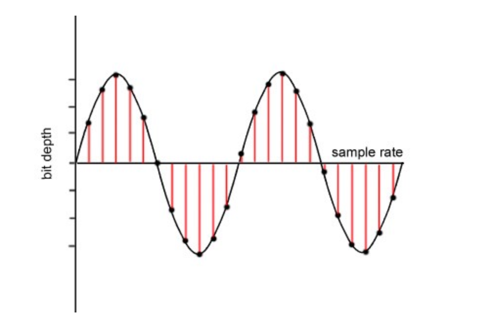
Amplitude

Amplitude is the magnitude or intensity of a sound wave. In simpler terms, it tells us how loud or soft a sound is. When you visualize an audio waveform, the amplitude is represented by the height of the waveform at any given point. In technical terms, amplitude is measured in decibels (dB) and represents the variation in air pressure caused by the sound wave. A higher amplitude corresponds to a greater variation in air pressure, resulting in a louder sound, while a lower amplitude indicates a softer sound. Amplitude is a fundamental characteristic of sound and plays a crucial role in how we perceive and interpret audio. It affects our perception of volume, dynamics, and overall sound quality. Understanding and controlling amplitude is essential in fields such as audio engineering, where precise control over sound levels is necessary to achieve desired outcomes in recording, mixing, and mastering audio tracks. Summary, amplitude is the measure of the intensity or loudness of a sound wave, expressed in decibels, and is a fundamental aspect of sound perception and audio signal processing.

Fourier Transform

The Fourier Transform is a mathematical tool used in signal processing to analyze and decompose complex signals into simpler components. Named after the French mathematician Joseph Fourier, who developed the concept in the early 19th century, it's a powerful technique that's widely used in various fields, including audio processing, image analysis, and telecommunications. At its core, the Fourier Transform works by breaking down a signal into its individual frequency components. You can think of it like breaking down a complex musical chord into its individual notes. By doing this, we can understand the different frequencies that make up the original signal and how much of each frequency is present. In practical terms, the Fourier Transform takes a time-domain signal, which represents the signal's amplitude over time, and converts it into a frequency-domain signal, which represents the signal's amplitude at different frequencies. This transformation allows us to analyze the frequency content of the signal and identify important features such as dominant frequencies, harmonics, and noise. There are different variants of the Fourier Transform, including the Discrete Fourier Transform (DFT) and the Fast Fourier Transform (FFT). The FFT is particularly popular because it allows for fast computation of the Fourier Transform, making it practical for real-time applications and digital signal processing. Fourier Transform is a mathematical technique used to analyze signals by breaking them down into their constituent frequency components. It's a fundamental tool in signal processing that's used to extract useful information from complex signals and has applications in various fields, including audio processing, telecommunications, and image analysis.

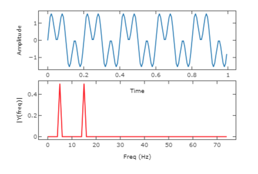
we will be using short time Fourier transform that is implemented in librosa. Fourier is an elegant way to decompose an audio signal into its constituent frequency.

Periodogram

The periodogram is a method used in signal processing to estimate the power spectrum of a signal. In simpler terms, it helps us understand the frequency content and power distribution of a signal. Imagine you have a signal, like a piece of music or a sound recording. The periodogram breaks down this signal into different frequency bands and tells us how much power or energy is present in each band. The process starts by dividing the signal into smaller segments, typically overlapping sections, to ensure that we capture all the frequency components accurately. Then, for each segment, we apply a Fourier Transform to convert the signal from the time domain to the frequency domain. This gives us a representation of the signal's frequency content. Next, we calculate the squared magnitude of the Fourier Transform for each segment. This squared magnitude represents the power or energy of the signal at each frequency. Finally, we average these squared magnitudes across all segments to obtain the periodogram, which shows us the distribution of power across different frequencies in the signal. The periodogram is useful for analyzing signals with varying frequency content, such as music or speech. It allows us to identify dominant frequencies, detect periodic patterns, and distinguish between signal and noise components. The periodogram is a method used in signal processing to estimate the power spectrum of a signal by analyzing its frequency content. It provides valuable insights into the characteristics of a signal and is widely used in fields such as audio processing, telecommunications, and vibration analysis.

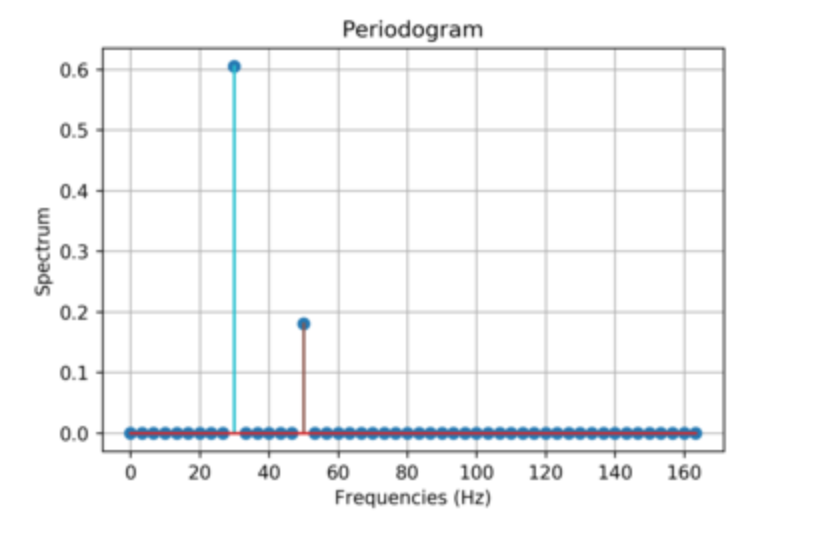
Spectral Density

Spectral density describes how the power of a signal is distributed across different frequencies. In simpler terms, it tells us how much power or energy is present in the signal at each frequency. Imagine you have a signal, like a piece of music or a sound recording. Spectral density helps us understand how much power or energy is concentrated in various frequency bands within that signal. Mathematically, spectral density is often represented as a function S(f) , where f represents frequency. This function describes the power or energy of the signal at each frequency f . In continuous-time signals, spectral density is typically represented in terms of power per unit frequency (e.g., watts per hertz), while in discrete-time signals, it's often represented in terms of power per unit frequency bin. The spectral density function provides valuable information about the frequency content of a signal. For example, it can help us identify dominant frequencies, detect periodic patterns, and distinguish between signal and noise components. By analyzing the spectral density of a signal, we can gain insights into its characteristics and better understand its underlying properties. Spectral density estimation is a common task in signal processing, and various techniques, such as the periodogram, Welch's method, and multitaper methods, are used to estimate spectral density from sampled data. These methods allow us to analyze the frequency content of signals in both time and frequency domains, enabling us to extract useful information and make informed decisions in various applications, including audio processing, telecommunications, and vibration analysis.

Mel-Scale

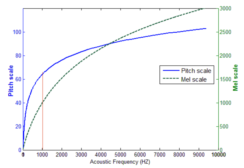
The Mel scale is a perceptual scale that maps frequencies to pitches in a way that approximates the human auditory system's response to different frequencies. Named after the scientist Steven Mels, it's widely used in audio signal processing, particularly in fields like speech recognition and music analysis. Here's how it works: The Mel scale is based on the idea that our perception of pitch is not linearly related to the actual frequency of a sound. Instead, we're more sensitive to changes in pitch at lower frequencies compared to higher frequencies. For example, we can easily distinguish between two tones that are an octave apart at low frequencies, but the same difference is less noticeable at higher frequencies. To account for this non-linear perception, the Mel scale uses a transformation that compresses lower frequencies and expands higher frequencies. This transformation is achieved through a series of mathematical operations, resulting in a scale where equal intervals correspond to equal perceptual differences in pitch. The formula for converting from frequency f to Mel scale m is typically given by: $$ m = 2595 \log_{10}(1 + \frac{f}{700}) $$ Conversely, to convert from Mel scale back to frequency, we use the inverse formula: $$ f = 700 (10^{\frac{m}{2595}} - 1) $$ The Mel scale is particularly useful in audio processing tasks where human perception of sound is important, such as speech recognition and music analysis. By using the Mel scale, we can design algorithms and systems that better mimic the way humans perceive and process auditory information, leading to improved performance and accuracy in these applications.

Cepstrum

The cepstrum is a powerful technique used in signal processing to analyze the spectral characteristics of a signal by examining its frequency components in a unique way. The term "cepstrum" is derived from "spectrum" spelled backward, highlighting its relationship with spectral analysis. Here's how it works: Calculate the Fourier Transform: The first step in computing the cepstrum involves taking the Fourier Transform of the signal. This converts the signal from the time domain to the frequency domain, revealing its frequency content. Take the Logarithm: Next, we take the logarithm of the magnitude spectrum obtained from the Fourier Transform. This helps to emphasize the relative amplitudes of different frequency components. Inverse Fourier Transform: After taking the logarithm, we perform an inverse Fourier Transform on the resulting spectrum. This converts the spectrum back from the frequency domain to the time domain. Cepstrum: The resulting signal is known as the cepstrum. It represents the "quefrency" domain, which is the domain of the inverse Fourier Transform of the logarithm of the spectrum. In other words, it captures information about the rate of change of the spectral components of the original signal.

Spectrogram

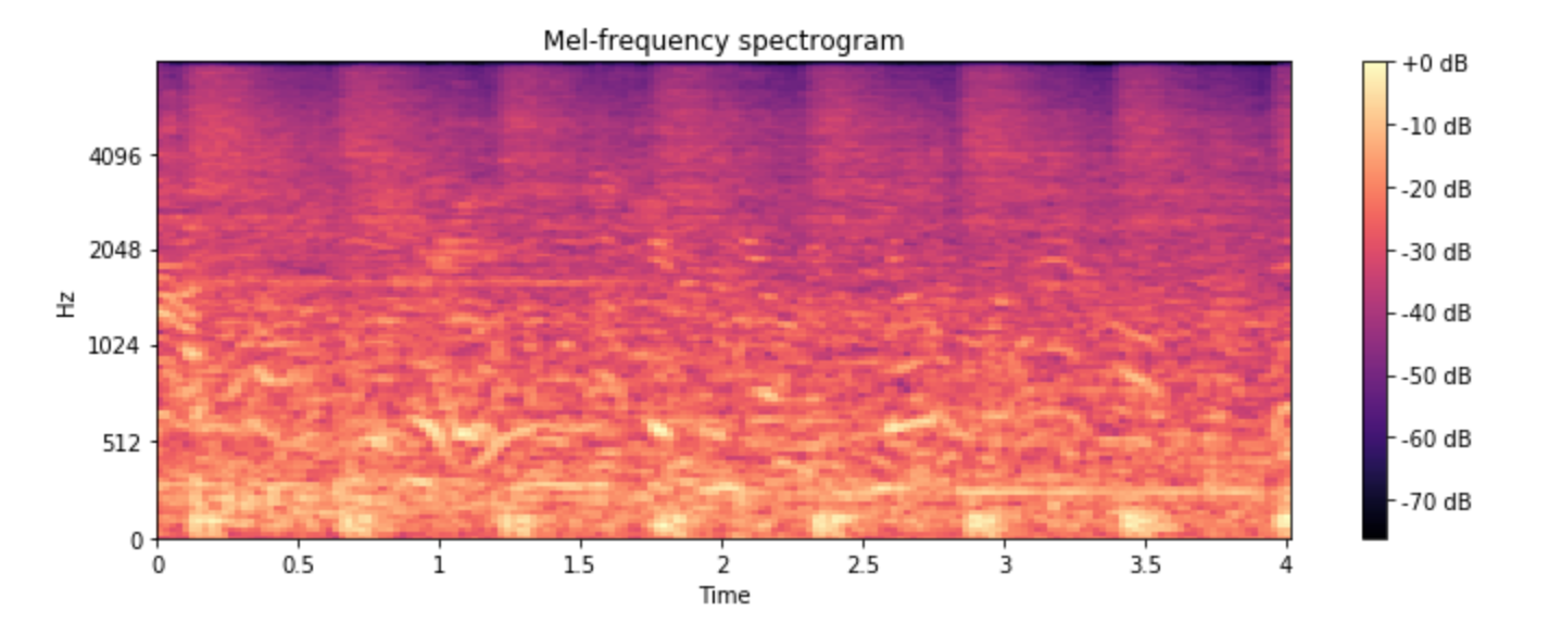
A spectrogram is a visual representation of the frequency content of a signal as it changes over time. It's like taking a snapshot of the frequency components of a signal at different moments and stitching them together to create a dynamic picture. Here's how it's done: Dividing the Signal: First, we divide the signal into small segments, typically using a technique called windowing. Each segment represents a short duration of the signal, such as a fraction of a second. Applying the Fourier Transform: Next, we apply the Fourier Transform to each segment. This converts the signal from the time domain to the frequency domain, revealing its frequency content. Power Spectrum Calculation: We then calculate the power spectrum of each segment. This tells us how much power or energy is present at each frequency within that segment. Building the Spectrogram: Finally, we arrange the power spectra of all segments over time to create the spectrogram. Typically, the horizontal axis represents time, the vertical axis represents frequency, and the intensity or color represents the power or energy level at each frequency and time point. In summary, spectrograms are a valuable tool for understanding the frequency content and temporal evolution of signals, enabling us to uncover patterns, identify features, and extract meaningful information from audio and other types of signals.

Convolutional Neural Network Blog

RNN & LSTM Blog

The deep learning concepts like CNN and RNN can be a different article. Please use the link to understand those concepts.

Methodologies

First we process the audio signal by extracting Mel-frequency cepstral coefficients (MFCCs) from audio smaples per-frame basis. The MFCC summarizes the frequency distribution over window size that enables us to analyze the frequency and features for classification. Once the preprocessing is complete we use CNN and RNN for classificatoin. However, this report particularly focuses on audio signal processing part.

That Dataset is taken from Kaggle. It consists of 300 audio samples and 10 different class labels with instrument.csv file.

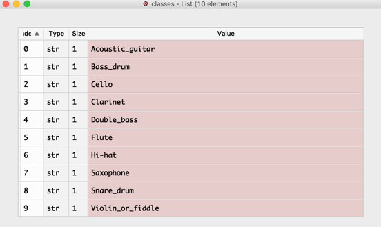
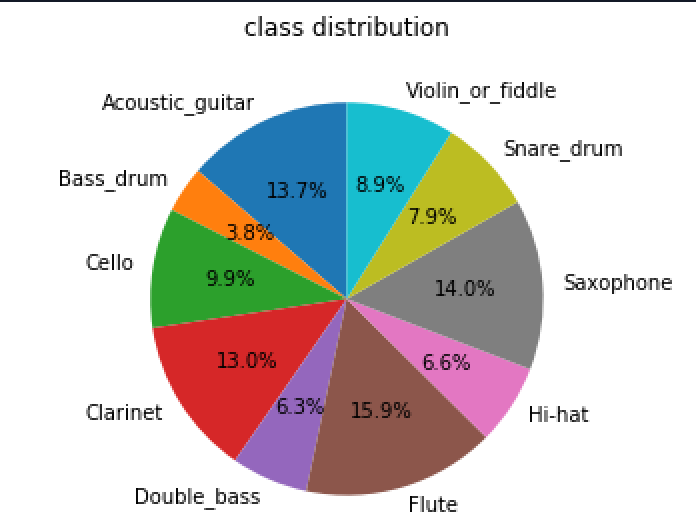
Lets further discuss the tools setup and pre-processing audio data. The dataset is 16-bit PCM and sampling rate of 44.1 kHz (44100 samples per second). The primary purpose is to compute MFCC and spectrogram of the audio signals. The audio signals are already preprocessed for window function which includes pre-emphasis, and framing.

Fourier Transform

Lets convert the time domain audio signal to frequency domain.

def calculate_fft(signal, rate):
    """"
    @params: signal, and sampling rate
    @return: mean normalized magnitude, and transformed frequency
    """"

    signal_length = len(signal)
    frequency = np.fft.rfftfreq(signal_length, d = 1/rate)
    #mean normalization of length of signal
    magnitude = abs(np.fft.rfft(signal)/signal_length) 
    return (magnitude, frequency)

Mel-Scale

We first compute filter bank using triangular filter. By default, the number of filters in Mel-scale are 40. For this instnace, lets use 26 standard filters to compute filter bank.

from python_speech_features import mfcc, logfbank
logfbank(signal[:rate], rate, nfilt=26, nfft=512)

The above function produces the array of size filter (26) by nfft i.e. 512 (default). Lets examine the coefficients for all classes.

The spectogram seems correlated among classes that leads deep learning models to confusion. Lets correct them by applying discrete cosine transformation as it decorrelates the filter bank coefficient and yields a compressed representation of filter banks. The spectral dimension is 26 by 512, lets reduce the size to 13 by 99 cepstral coefficients because fast changing filter bank coefficients do not carry additional information. New spectogram of 13 by 99 looks following.

Now, we have input ready for CNN and RNN to classify instruments. The input size of each instance is 13 by 99. From this point, i will let you to use Tensorflow or pytorch to build deep learning models. Code

Conclusion

We explored the audio signal processing for deep learning models. Since, the development of LLM models, CNN and RNNs are frivolus. The GenAI has ability to create and compose music. The main objective of this article is to provide the understanding the basic pieces od audio signals, and will definately bolsters use them in GenAI.

References

Kaggle

Speech processing for machine learning

Mel Frequency Cepstral Coefficient (MFCC) tutorial